1. 热等离子体为什么会发 X 射线?
1. Why does hot plasma emit X-rays?
百万度(kT ≈ 0.1–1 keV,1 keV ≈ 1.16×10⁷ K)的稀薄气体里,电子被离子加速时发出轫致辐射(thermal bremsstrahlung),形成随能量平滑下降的连续谱;同时离子的内层电子被碰撞激发再退激发,发出尖锐的谱线。对 0.3–1 keV 的晕气体,最重要的是铁的 L 复合线(Fe-L complex,约 0.7–1.2 keV):它的位置和强度随温度变化很快,是测 kT 的主要信息来源。
In gas at millions of degrees (kT ≈ 0.1–1 keV; 1 keV ≈ 1.16×10⁷ K), electrons accelerated by ions emit thermal bremsstrahlung — a continuum falling smoothly with energy — while collisionally excited ions emit sharp spectral lines. For 0.3–1 keV halo gas the most important feature is the iron L complex (Fe-L, ≈ 0.7–1.2 keV): its position and strength change rapidly with temperature, and it carries most of the kT information.
算一个数:kT = 0.75 keV 的气体,Fe-L 线附近(0.7–1.05 keV)光子最多,因为 e^(−E/kT) 还没衰减太多而 Fe-L 正好在峰上。温度升到 1.2 keV,整个谱变硬(更平),Fe-L 相对变弱。下面的图用玩具模型演示这一点(不是真实 APEC,只示意)。
A quick number: for kT = 0.75 keV gas, photons near the Fe-L band (0.7–1.05 keV) dominate, because e^(−E/kT) has not fallen much while Fe-L sits on the peak. Raise the temperature to 1.2 keV and the spectrum hardens (flattens) while Fe-L weakens relatively. The figure below shows this with a toy model (illustrative, not the real APEC).
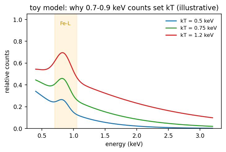
三个温度的玩具谱。橙色带是 Fe-L 复合线所在能段。 Toy spectra at three temperatures. The orange band marks the Fe-L complex.
fig_scripts/make_figures.py(toy simulation,illustrative only)
2. APEC 模型与归一化 norm
2. The APEC model and its normalization
APEC 是天体物理标准的热等离子体光谱模型:给定温度 kT、金属丰度 Z(相对太阳)和红移,它给出单位发射量在每能量上的发射率。观测谱拟合时再乘一个归一化 norm:
APEC is the standard astrophysical thermal-plasma model: given kT, metallicity Z (relative to solar) and redshift, it gives the emissivity per unit emission measure as a function of energy. Fitting an observed spectrum multiplies it by a normalization:
norm = (10⁻¹⁴ / (4π [D_A(1+z)]²)) × ∫ n_e n_H dV (cm⁻⁵)
算一个数:M104 距离 D_A ≈ 9.55 Mpc = 2.95×10²⁵ cm,则 10⁻¹⁴/(4π D²) ≈ 9.1×10⁻⁶⁶。若拟合得 norm = 6×10⁻⁶ cm⁻⁵,则 ∫n_e n_H dV ≈ 6.6×10⁵⁹ cm⁻³。对一个体积 V ≈ (20 kpc)³ ≈ 4.7×10⁷¹ cm³ 的球,n_e ≈ √(6.6×10⁵⁹/4.7×10⁷¹) ≈ 1.2×10⁻⁶ cm⁻³ —— 正是星系晕气体的典型密度。
Worked example: M104 is at D_A ≈ 9.55 Mpc = 2.95×10²⁵ cm, so 10⁻¹⁴/(4π D²) ≈ 9.1×10⁻⁶⁶. If the fit gives norm = 6×10⁻⁶ cm⁻⁵, then ∫n_e n_H dV ≈ 6.6×10⁵⁹ cm⁻³. For a sphere of volume V ≈ (20 kpc)³ ≈ 4.7×10⁷¹ cm³, n_e ≈ √(6.6×10⁵⁹/4.7×10⁷¹) ≈ 1.2×10⁻⁶ cm⁻³ — a typical halo-gas density.
3. CCD 光谱与前向折叠(ARF ⊗ RMF)
3. CCD spectra and forward folding (ARF ⊗ RMF)
X 射线 CCD 探测器并不直接记录光子能量:它记录的是电荷量(PI 通道),能量分辨率有限(MOS 约 70 eV)。此外望远镜的有效面积随能量和离轴角变化(渐晕,vignetting)。因此理论模型必须“前向折叠”后才能与数据比较:
An X-ray CCD does not record photon energy directly: it records charge (PI channels) with limited resolution (~70 eV for MOS). The telescope effective area also varies with energy and off-axis angle (vignetting). So the model must be “forward folded” before comparing with data:
predicted counts(channel) = [model(E) × ARF(E)] ⊗ RMF(E→channel) + background
ARF(ancillary response file)是有效面积随能量的曲线;RMF(redistribution matrix file)把真能量映射到测量通道的概率矩阵。拟合就是调模型参数,让折叠后的预测计数与每通道观测计数在统计上最一致。
The ARF (ancillary response file) is the effective area as a function of energy; the RMF (redistribution matrix file) is the probability matrix mapping true energy to measured channel. Fitting adjusts model parameters so the folded prediction matches the counts in every channel as well as possible.
4. 背景成分:为什么外区几乎全是背景
4. Background components: why the outskirts are almost all background
XMM 谱里的计数远不止源:
The counts in an XMM spectrum are far from all source:
- QPB(quiescent particle background,静默粒子背景):探测器自身被宇宙线粒子激发,用滤光片关闭时(FWC, closed filter wheel)的观测建模;
- QPB (quiescent particle background): detector counts excited by cosmic-ray particles, modelled from closed-filter-wheel (FWC) observations;
- SP(soft proton,软质子):太阳活动抛出的质子在探测器上产生平坦的连续谱,需要用光变曲线剔除宁静期外的时间,模型上用幂律/broken powerlaw;
- SP (soft protons): solar protons producing a flat continuum on the detector; quiet periods are cut with light curves and the rest modelled with a (broken) powerlaw;
- 天空背景:LHB(local hot bubble,本地热泡)、MW halo(银河系晕)、CXB(cosmic X-ray background,宇宙 X 射线背景,未分辨遥远源)、SWCX(太阳风电荷交换);
- Sky background: LHB (local hot bubble), MW halo, CXB (cosmic X-ray background, unresolved distant sources), SWCX (solar-wind charge exchange);
- 仪器线:Al 1.49 keV、Si 1.75 keV 等探测器荧光线(v18 用经验高斯拟合)。
- Instrumental lines: Al 1.49 keV, Si 1.75 keV etc. (fitted as empirical Gaussians in v18).
算一个数(E030 实测):R4–7 北侧单扇区 11.62 arcmin²,Fe-L 能段 CGM 光子 62 个,背景 184 个 —— 源只占 25%。R6–8 Angle1 是 131/410(24%)。源越弱,kT 越容易被背景形状牵着走。
Worked example (measured in E030): the R4–7 north single sector, 11.62 arcmin², has 62 CGM photons vs 184 background photons in the Fe-L band — the source is 25%. R6–8 Angle1 is 131/410 (24%). The weaker the source, the more the fitted kT is dragged by the background shape.
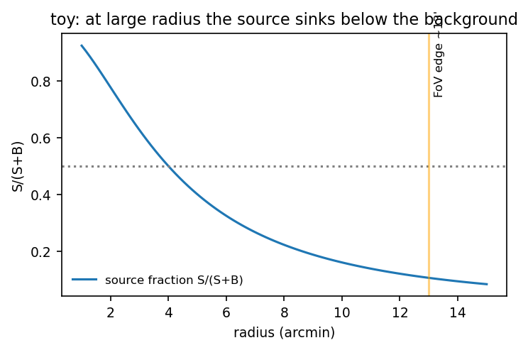
玩具图:源占比随半径下降。13′ 之后源几乎消失,拟合进入“背景决定温度”的退化区。 Toy: the source fraction falls with radius. Beyond ~13′ the source nearly vanishes and the fit enters the regime where the background dictates the temperature.
5. C 统计量与 profile likelihood 68% 区间
5. The C statistic and profile-likelihood 68% intervals
X 射线计数是泊松分布,所以用 Cash 的 C 统计量:
X-ray counts are Poisson-distributed, so we use Cash's C statistic:
C = 2 Σ [ m_i − y_i + y_i ln(y_i / m_i) ]
其中 y_i 是第 i 通道观测计数,m_i 是模型预测。拟合使 C 最小。参数 θ 的 68% 区间由 ΔC = 1 定义:固定 θ 于候选值、重新优化所有其他参数(profile),C 上升 1 的两个 θ 即区间端点。算一个数:若 kT = 0.70 时 C = 130.98,kT = 0.637 与 kT = 0.729 时 C 都 = 131.98,则 68% 区间是 [0.637, 0.729] —— 这正是 E030 R2–4 Angle1 的实测结果(0.684 keV,区间 0.637–0.729,最大相对误差 6.9%)。
where y_i is the observed count in channel i and m_i the model prediction; the fit minimizes C. The 68% interval of a parameter θ is defined by ΔC = 1: fix θ at a candidate value, re-optimize all other parameters (profiling), and the two θ where C rises by 1 are the interval ends. Worked example: if C(0.70) = 130.98 while C(0.637) and C(0.729) both equal 131.98, the 68% interval is [0.637, 0.729] — exactly the measured E030 R2–4 Angle1 result (0.684 keV, interval 0.637–0.729, max relative error 6.9%).
analysis_plans/m104_temperature_area_20261005/actual_src_bkg_results_zh.md(表格第一行)
弱信号区的陷阱(Q-C 的根源)。当源占比低时,温度与背景归一化强烈简并:拟合可以让“源更冷+背景更少”或“源更热+背景更多”给出几乎相同的 C。于是 kT 可能落到参数边界(如 0.46 keV 触下限)或跑出非物理值。v18 表中 R12-14_Angle1 的通量 ≈ 4×10⁻²¹ erg s⁻¹ cm⁻² arcmin⁻²(塌缩)、kT = 0.456 触边界,就是这类失败的实例。参数边界不是误差棒。
The weak-signal trap (the root of Q-C). When the source fraction is low, temperature and background normalizations are strongly degenerate: “colder source + less background” and “hotter source + more background” can give nearly the same C. The fitted kT can then hit a parameter bound (e.g. 0.46 keV at the lower limit) or run to unphysical values. In the v18 table, R12-14_Angle1 has flux ≈ 4×10⁻²¹ erg s⁻¹ cm⁻² arcmin⁻² (collapsed) with kT = 0.456 at the bound — a textbook failure. Parameter bounds are not error bars.
给大一学生的 B020 单位课(一个算例)。读数前先问:“这个数是总量还是单位面积的量?”v18 拟合脚本把所有天空成分乘上 skyarea = BACKSCAL·(1/20/60)² arcmin²,所以保存的 flux_0.5-2.0keV 已经是每 arcmin² 的面亮度(erg s⁻¹ cm⁻² arcmin⁻²)。算一个数:R11-13_Angle2 的保存值是 8.82×10⁻¹⁶ erg s⁻¹ cm⁻² arcmin⁻²。旧轮廓又除了一次几何面积 75.4 arcmin²,得到 1.17×10⁻¹⁷ erg s⁻¹ cm⁻² arcmin⁻² arcmin⁻²——单位里出现了两个 arcmin⁻²!小面积的外侧 bin 被抬高得最多,看起来就像 13′ 处有个“亮环”。修正后(裸面亮度)11–14′/8–11′ = 1.37 而不是 1.04 的相反信号,且独立图像不显示任何超出(I065)。教训:比较两个数之前,先写下每个数的单位和产生它的代码行。
B020's units lesson for a first-year student (one worked number). Before using a number, ask: “is this a total or a per-unit-area quantity?” The v18 fitting script multiplies every sky component by skyarea = BACKSCAL·(1/20/60)² arcmin², so the saved flux_0.5-2.0keV is already a surface brightness per arcmin² (erg s⁻¹ cm⁻² arcmin⁻²). Worked example: R11-13_Angle2's saved value is 8.82×10⁻¹⁶ erg s⁻¹ cm⁻² arcmin⁻². The old profiles divided it once more by the geometric area, 75.4 arcmin², giving 1.17×10⁻¹⁷ erg s⁻¹ cm⁻² arcmin⁻² arcmin⁻² — two arcmin⁻² in the units! The small-area outer bins get inflated the most, which looked like a “bright ring” at 13′. With the bare surface brightness the 11–14′/8–11′ ratio is 1.37 rather than the opposite signal at 1.04, and the independent images show no excess at all (I065). Lesson: before comparing two numbers, write down each one's units and the code line that produced it.
v18_profile_analysis/v18_complete_parameters.csv(regionR12-14_Angle1 行);cognition-os/bug_impacts/B020_*.md;cognition-os/insights/I065_*.md;joint_spectrum_fitting_2T_basedon_region_v18.py:951–966, 2014–2029
6. Chandra vs XMM:联合拟合得到什么
6. Chandra vs XMM: what joint fitting gains
| 特性Property | XMM-Newton EPICXMM-Newton EPIC | Chandra ACISChandra ACIS | |||
|---|---|---|---|---|---|
| 角分辨率(PSF) | Angular resolution (PSF) | ~6″ (HEW) | ~0.5″ | ||
| 有效面积 | Effective area | 大(三相机合计 ~0.4 m² @1 keV)→ 光子多 | Large (three cameras, ~0.4 m² at 1 keV) → many photons | 小 → 光子少 | Small → fewer photons |
| 背景 | Background | SP 粒子污染显著 | Strong soft-proton contamination | 粒子背景低且可精确建模 | Low, well-modelled particle background |
| 强项 | Strength | 弱扩展源的精度 | Precision on faint extended sources | 分辨点源/AGN、控制污染 | Resolving point sources/AGN, contamination control |
联合拟合(J1/J2)让两个仪器共享源物理参数(kT、Z),但各自保留自己的响应与背景模型。理论上区间更紧;但 E031 核验发现:严格“所有仪器都有支持”的天空交集在 R6–8 只剩 5.2% 面积,弱信号使联合 profile 出现双分支(0.14–0.20 与 1.5–5.9 keV)——更紧的区间若来自系统分歧而非一致信息,就不是确认。
Joint fitting (J1/J2) shares the source physics (kT, Z) between instruments while each keeps its own response and background. In principle the interval tightens; but E031 found that the strict “all instruments support this sky” intersection keeps only 5.2% of the R6–8 annulus, and the weak signal makes the joint profile bimodal (0.14–0.20 vs 1.5–5.9 keV) — a tighter interval that comes from unresolved disagreement rather than consistent information is not confirmation.
analysis_plans/m104_temperature_area_20261005/m104_temperature_map_delivery_strategy_zh.md;cognition-os/experiments/E031_*.md